Grohe Smarthome (Sense and Blue) integration for Home Assistant
This is an integration for all the Grohe Smarthome devices into Home Assistant. Namely, these are:
Grohe Sense (small leak sensor)
Grohe Sense Guard (main water pipe sensor/breaker)
Grohe Blue Home (water filter with carbonation)
Grohe Blue Professional (water filter with carbonation)
Disclaimer
The authors of this integration are not affiliated with Grohe or the Grohe app in any way. The project depends on the undocumented and unofficial Grohe API. If Grohe decides to change the API in any way, this could break the integration. Even tough the integration was tested on several devices without problems, the authors are not liable for any potential issues, malfunctions or damages arising from using this integration.
Use at your own risk!
Getting started
If you’re new, take a look at the Installation Guide here: Getting Started
Other documentation for available actions, device sensors, notifications, etc. can be found in the wiki
Remarks on the “API”
I have not seen any documentation from Grohe on the API this integration is using, so likely it was only intended for their app.
Breaking changes have happened previously, and can easily happen again.
I try to always keep the integration updated to their latest API.
The API returns much more detailed data than is exposed via these sensors.
For withdrawals, it returns an exact start- and end time for each withdrawal, as well as volume withdrawn.
It seems to store data since the water meter was installed, so you can extract a lot of historic data (but then polling gets a bit slow).
I’m not aware of any good way to expose time series data like this in home assistant (suddenly I learn that 2 liters was withdrawn 5 minutes ago, and 5 liters was withdrawn 2 minutes ago).
If anyone has any good ideas/pointers, that’d be appreciated.
Credits
Thanks to:
gkreitz for the initial implementation of the Grohe Sense
rama1981 for reaching out and going through the trial and error for the Grohe Blue Professional.
daxyorg for going through the trial and error of the refactored version and testing with Grohe Blue Home.
windkh from whom I’ve token a lot of the notification types available.
Laravel is a web application framework with expressive, elegant syntax. We believe development must be an enjoyable and creative experience to be truly fulfilling. Laravel takes the pain out of development by easing common tasks used in many web projects, such as:
Laravel is accessible, powerful, and provides tools required for large, robust applications.
Learning Laravel
Laravel has the most extensive and thorough documentation and video tutorial library of all modern web application frameworks, making it a breeze to get started with the framework.
You may also try the Laravel Bootcamp, where you will be guided through building a modern Laravel application from scratch.
If you don’t feel like reading, Laracasts can help. Laracasts contains over 2000 video tutorials on a range of topics including Laravel, modern PHP, unit testing, and JavaScript. Boost your skills by digging into our comprehensive video library.
Laravel Sponsors
We would like to extend our thanks to the following sponsors for funding Laravel development. If you are interested in becoming a sponsor, please visit the Laravel Patreon page.
Thank you for considering contributing to the Laravel framework! The contribution guide can be found in the Laravel documentation.
Code of Conduct
In order to ensure that the Laravel community is welcoming to all, please review and abide by the Code of Conduct.
Security Vulnerabilities
If you discover a security vulnerability within Laravel, please send an e-mail to Taylor Otwell via taylor@laravel.com. All security vulnerabilities will be promptly addressed.
License
The Laravel framework is open-sourced software licensed under the MIT license.
WARNING: Please note that this project is intended as an illustrative example of the potential application of machine learning in assisting medical professionals with heart disease diagnosis. The information and results presented here (or on the accompanying website) do not constitute medical advice in any form.
Heart disease is a prevalent health condition that requires accurate and timely diagnosis for effective treatment. This project aims to develop a machine learning model to assist doctors in diagnosing heart disease accurately and efficiently. By leveraging statistical learning algorithms and a comprehensive dataset, the model can analyze various patient factors and provide predictions regarding the probability of heart disease. The implementation of diagnostic machine learning models like this one offers several potential benefits, including improved diagnostic accuracy, reduced burden on medical professionals, and early detection of disease. Furthermore, the project promotes data-driven medicine and contributes to ongoing efforts in machine learning-based medical diagnosis. By providing an additional tool for risk assessment and decision-making, I hope that models like this one can enhance patient outcomes and advance our understanding of heart disease.
Usage
Please note that the Heart Disease Prediction Website is intended for demonstration and educational purposes only and should not substitute professional medical advice or diagnosis.
A medical professional could collect and enter the necessary patient information (such as age, sex, chest pain type, resting blood pressure, etc.) into the website
Once all the required data has been entered, click the “Predict” button to initiate the prediction process.
A medical professional could interpret the prediction result alongside other diagnostic information and medical expertise to make informed decisions and provide appropriate care for the patient.
RestingECG: resting electrocardiogram results [Normal: Normal, ST: having ST-T wave abnormality (T wave inversions and/or ST elevation or depression of > 0.05 mV), LVH: showing probable or definite left ventricular hypertrophy by Estes’ criteria]
MaxHR: maximum heart rate achieved [Numeric value between 60 and 202]
Oldpeak: oldpeak = ST [Numeric value measured in depression]
ST_Slope: the slope of the peak exercise ST segment [Up: upsloping, Flat: flat, Down: downsloping]
HeartDisease: output class [1: heart disease, 0: Normal]
Source
This dataset was created by combining different datasets already available independently but not combined before. In this dataset, 5 heart datasets are combined over 11 common features which makes it the largest heart disease dataset available so far for research purposes. The five datasets used for its curation are:
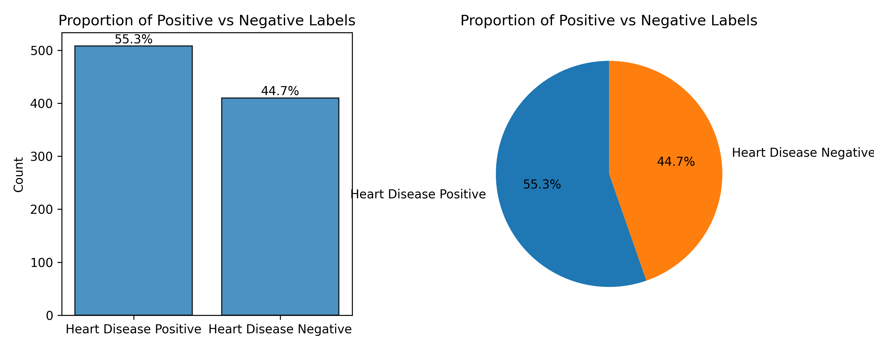
How many positive and negative examples are there of the target variable?
The dataset is close to balanced, so there is no need to impliment techniques to improve classifaction of infrequent categories like Synthetic Minority Over-sampling.
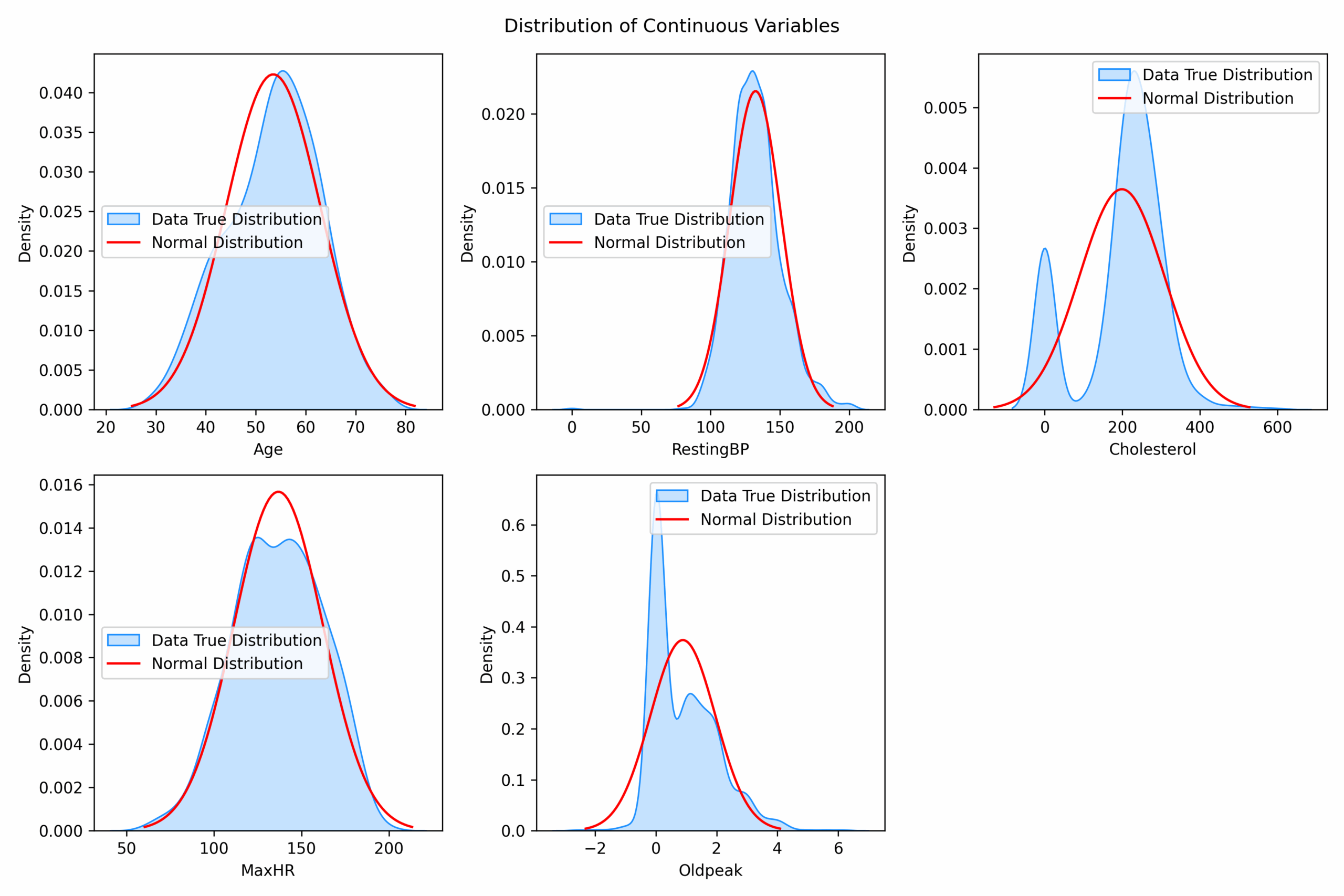
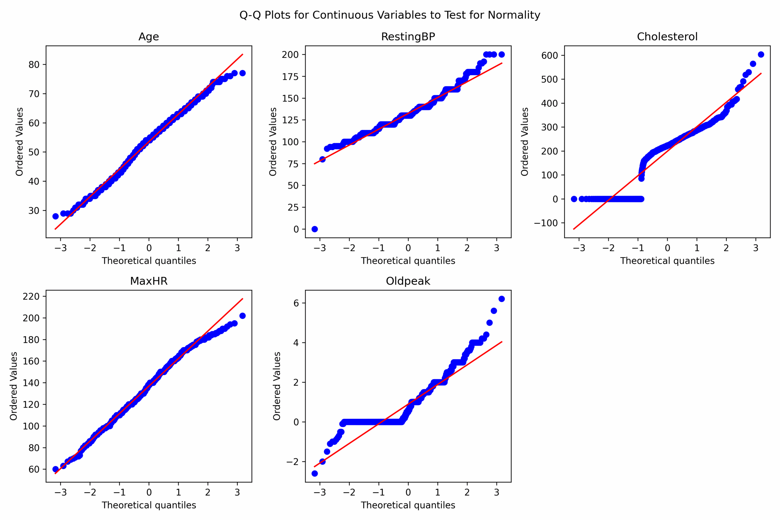
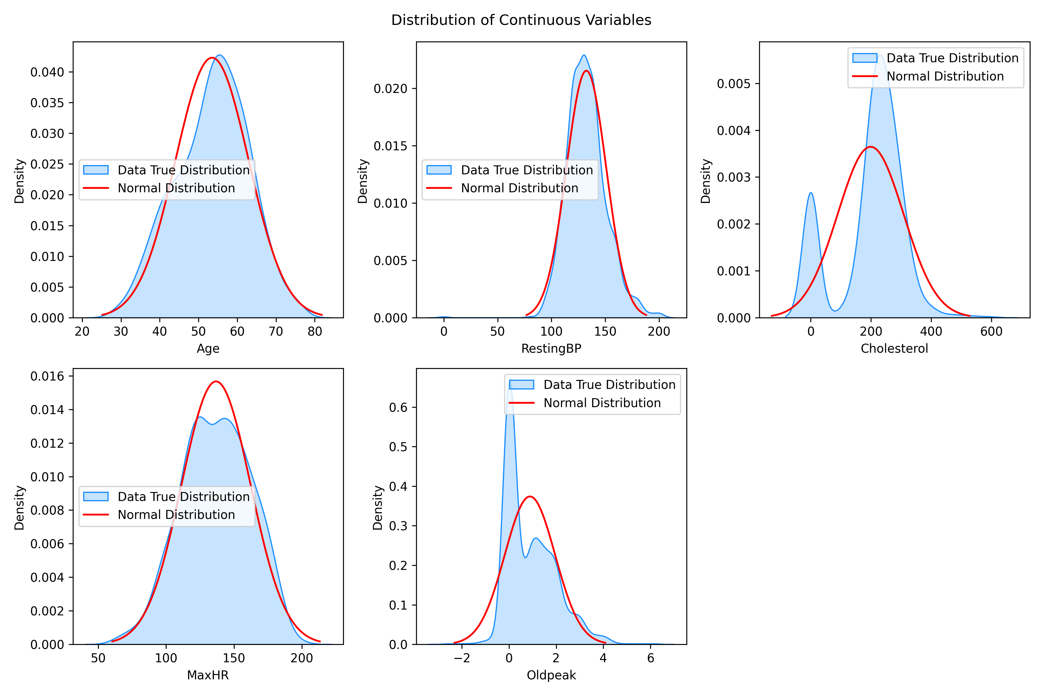
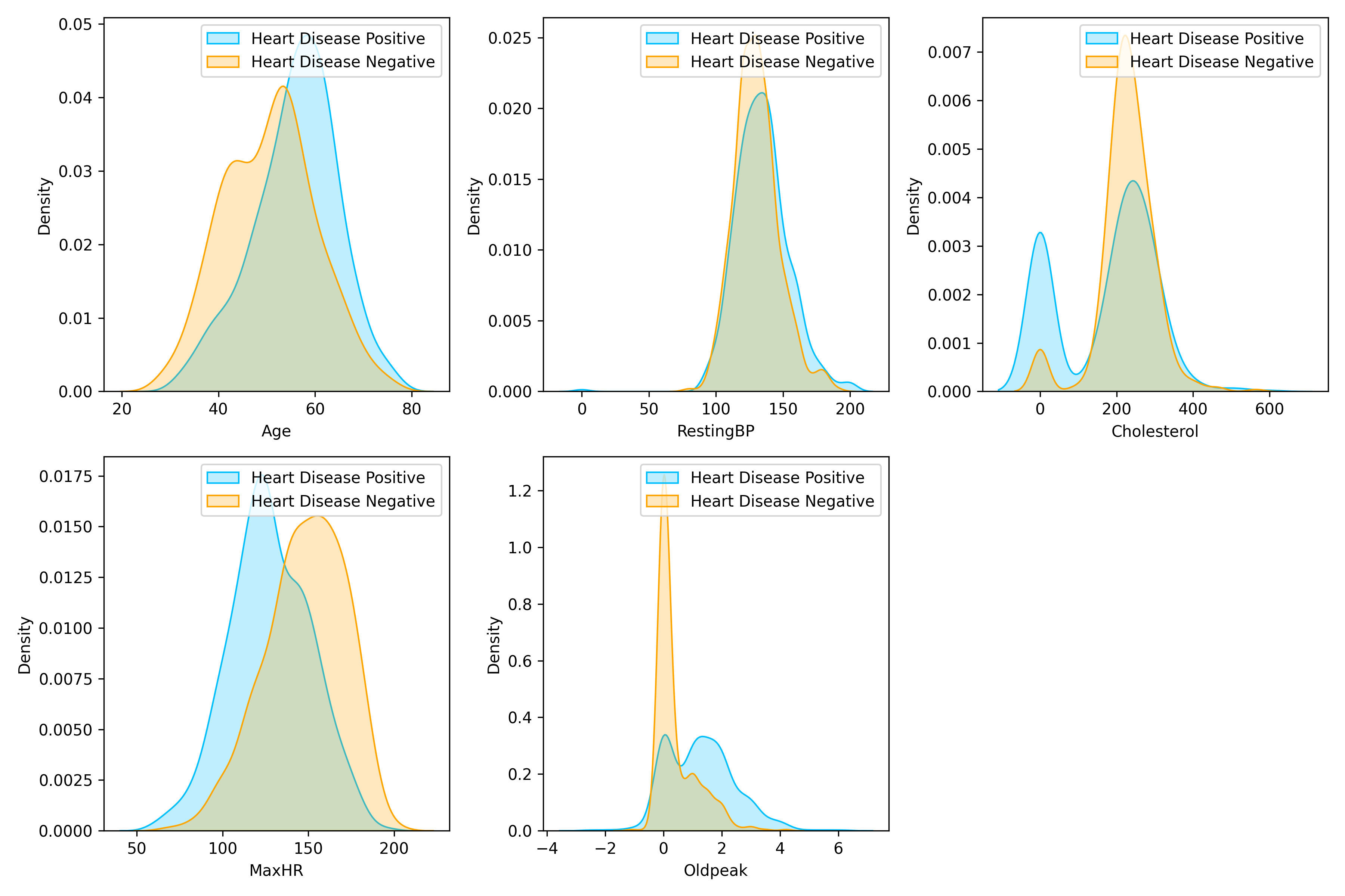
How are continuous variables distributed (in particular, are they normally distributed)?
Key Takeaways:
Upon visually examining the distribution of age, resting blood pressure, and maximum heart rate, they appeared to resemble a normal distribution. However, the application of Q-Q plots indicated deviations from Gaussian distribution. Consequently, I conducted Shapiro-Wilk tests on each of these variables, which confirmed their non-normal distribution.
Notably, a considerable number of cholesterol values were assigned as 0 to represent null values.
Leveraging These Insights:
To address the departure from normality, I opted to employ the StandardScaler() function from the sklearn library. This transformation aimed to bring the data points closer to a normal distribution.
Initially, when constructing the baseline models, I retained the original cholesterol data without any modifications. However, to overcome the limitation imposed by the null cholesterol values, I employed a series of techniques which aim to replace the null values with numbers from which models can generate meaningful predictions.
How do continuous variables change in conjunction with the target variable?
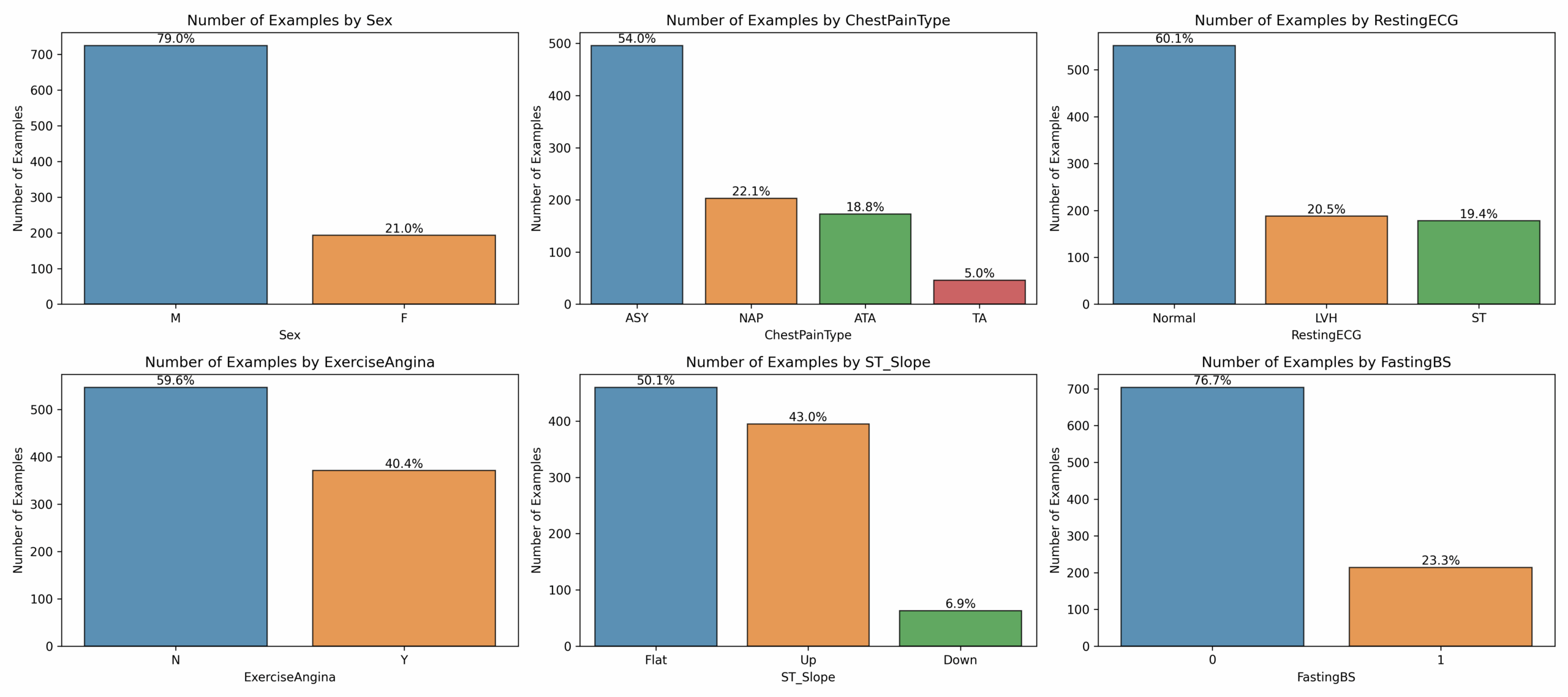
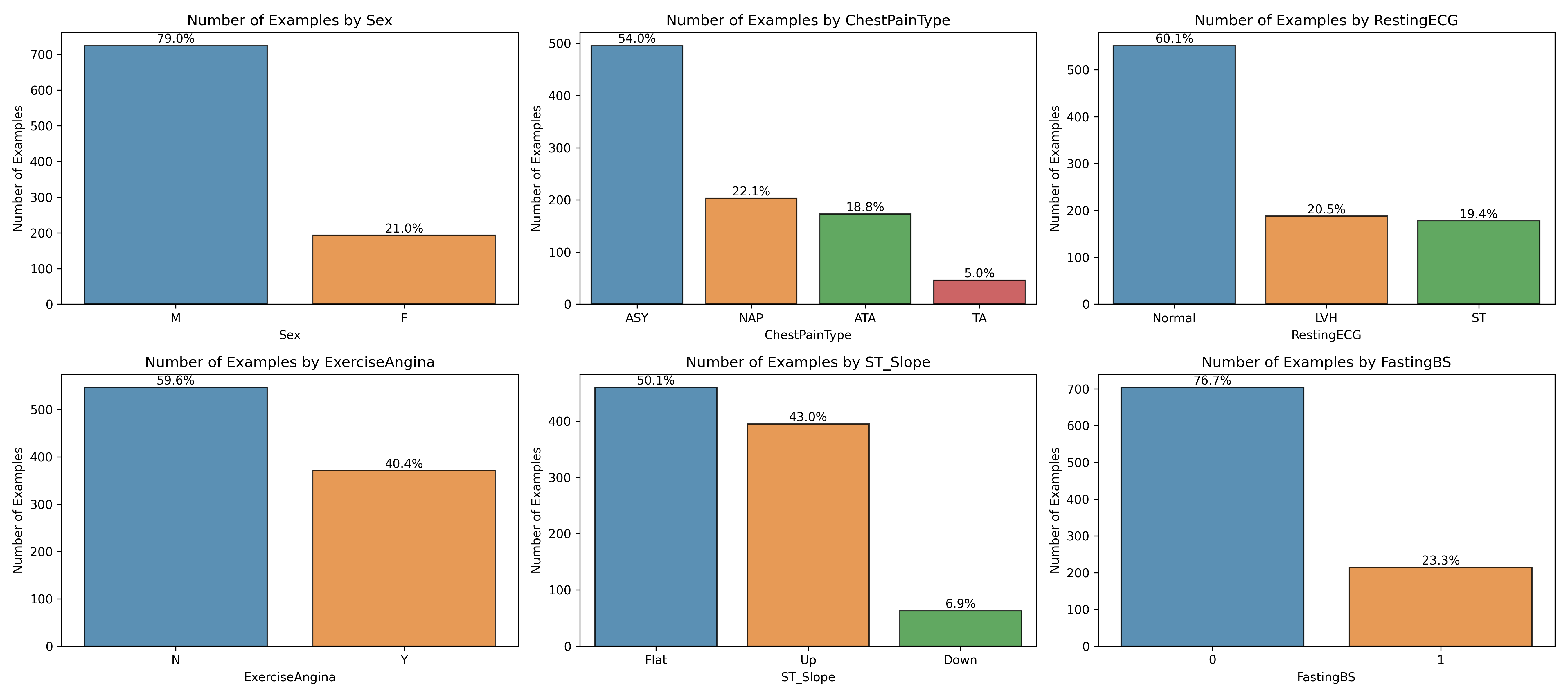
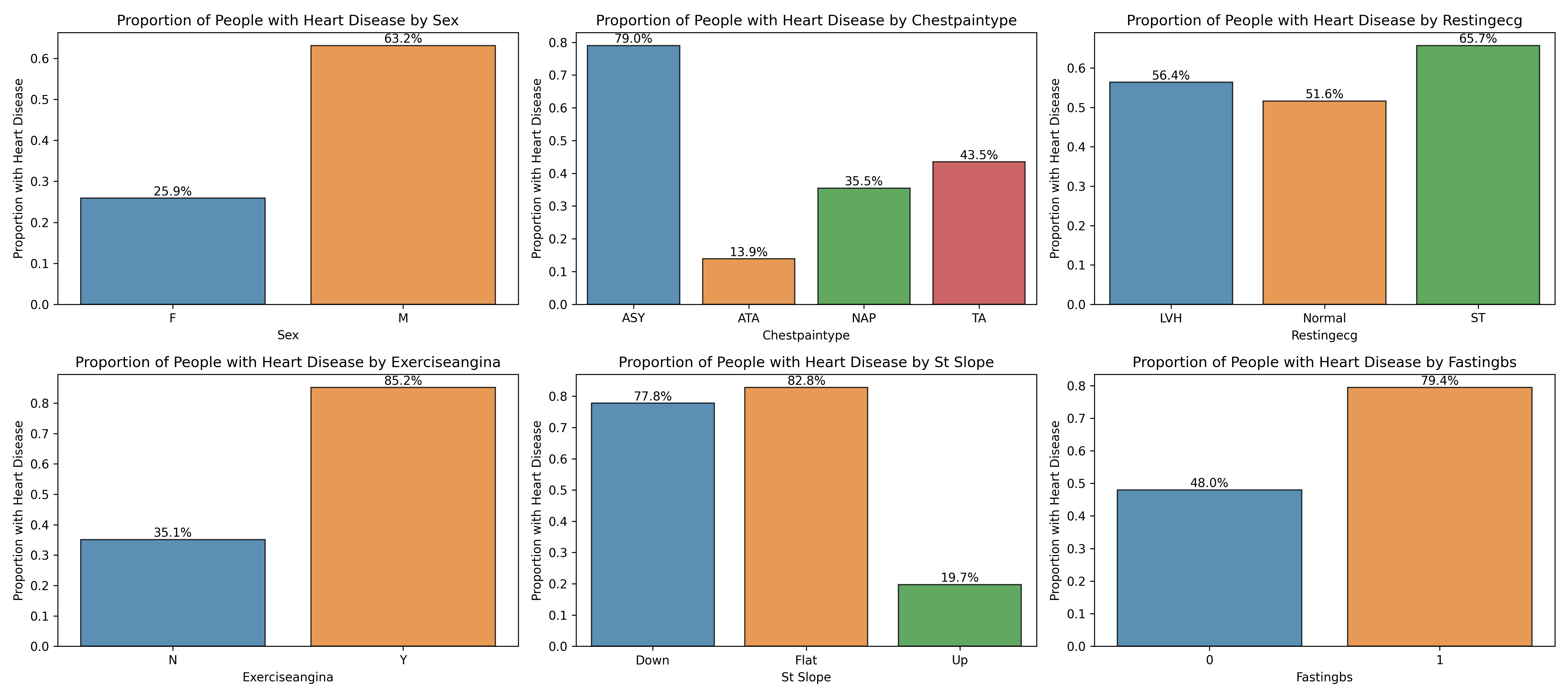
How many examples are there of each categorical variable?How does each categorical variable change in conjunction with the target variable?
Feature Selection With Inferential Statistics
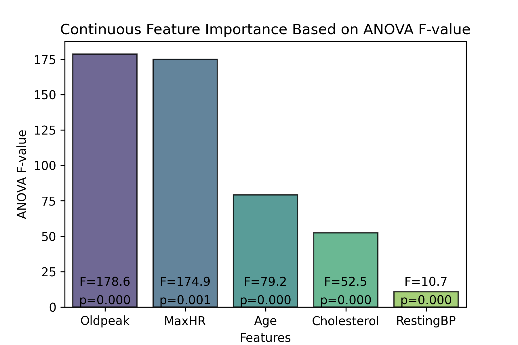
I used inferential statistics to determine the importance of the dataset’s features. If I found that a feature has no significant impact on the target variable, then it would be helpful to try models which discard that variable. Removing an insignificant vairbale would reduce noise in the data, ideally lowering model overfitting and improving classification accuracy. For continuous features, I conducted an ANOVA, and for categorical features, I used a Chi-Squared Test.
ANOVA
Analysis of Variance (ANOVA) is a method from inferential statistics that aims to determine if there is a statistically significant difference between the means of two (or more) groups. This makes it a strong candidate for determining importance of continuous features in predicting a categorical output. I used a One-Way ANOVA to test the importance of each continuous feature by checking whether presence of heart disease had a statistically significant effect on the feature’s mean.
ANOVA Results
I found that there was a statistically significant difference (p<0.05) for each continuous feature. This led me to decide to keep all continuous features as part of my classification models.
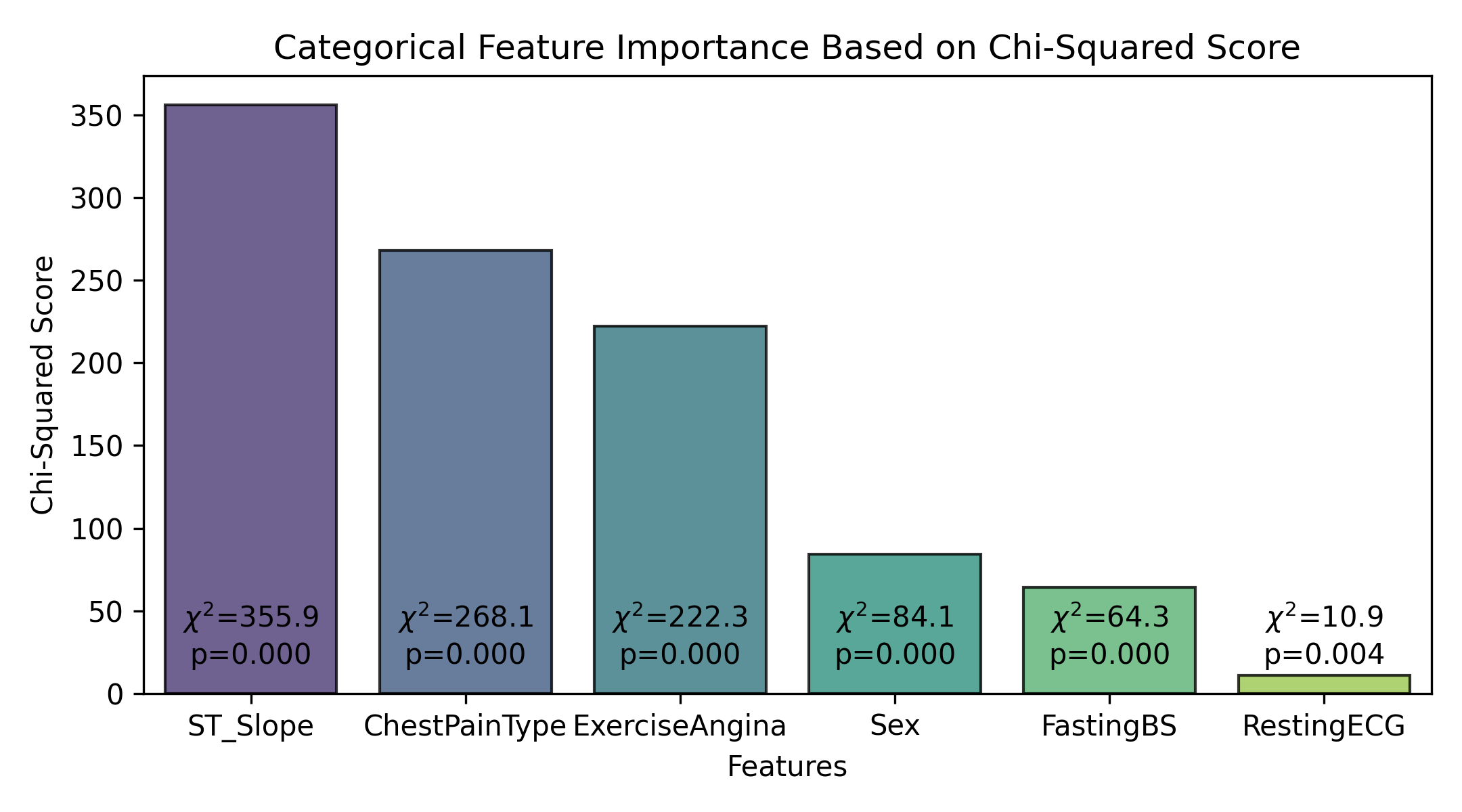
Chi-Squared Test
The Chi-Squared test is a statistical hypothesis test that is used to determine whether there is a significant association between two categorical variables. It compares the observed frequencies in each category of a contingency table with the frequencies that would be expected if the variables were independent. In the context of feature selection for my machine learning models, I used the Chi-Squared test to identify the categorical features that are most significantly associated with the target variable.
Chi-Squared Test Results
Like the continuous features, I found a statistically significant difference in heart disease (p<0.05) according to each categorical feature. This led me to decide to keep all categorical features as part of my classification models.
Data Imputation Techniques for Null Value Replacement
As I discovered during Exploratory Data Analysis, the dataset has 172 samples with null values for Cholesterol (which were initially set to 0). I explored various data imputation techniques in an attempt to extract meaningful training data from such samples.
Initially, simple imputation strategies were deployed, namely: mean, median, and mode imputation. A noteworthy improvement in model performance was observed compared to models trained on the original dataset where null values were replaced by a default value of zero. Among these initial imputation techniques, mean imputation was found to deliver the best results for most machine learning models.
Building upon these initial findings, I applied a sophisticated imputation method: applying regression analysis to estimate the missing values. The regression techniques applied included Linear Regression, Ridge Regression, Lasso Regression, Random Forest Regression, Support Vector Regression, and Regression using Deep Learning. Each of these regression-based imputation techniques displayed a similar level of performance in terms of RMSE and MAE.
The performance of the regression models was found to be not as satisfactory as initially hypothesized, often falling short of the results obtained with mean imputation. Despite this, it was observed that for Random Forest Classifiaction models, the regression-based methods exhibited strong results in terms of precision and specificity metrics. Particularly, Linear Regression and Ridge Regression-based imputation strategies performed well in these areas.
Classification Models
A key component of this project involved the implementation and performance evaluation of a variety of classification models. The chosen models were tested on the datasets prepared as described in the “Data Imputation Techniques for Null Value Replacement” section. All the datasets utilized in this phase had continuous features standardized and normalized to ensure a uniform scale and improved model performance.
Logistic Regression
Random Forest Classifier
Support Vector Machine Classifier
Gaussian Naive Bayes Classifier
Bernoulli Naive Bayes Classifier
XGBoost Classifier
Neural Network (of various architectures)
For the neural network models, an expansive exploration of hyperparameter variations was conducted using cross-validation. These architectures ranged from those with a single hidden layer to those with three hidden layers, with the number of neurons per layer varying from 32 to 128.
Each of these models was trained on 80% of the data, and tested on 20%. Accuracy, Precision, Recall, F1-Score and Specificity metrics were tracked.
Results and Model Performance Evaluation
A thorough analysis of over 80 models was conducted in this project, with the evaluation criteria based on several metrics including accuracy, precision, recall (sensitivity), F1-score, and specificity. Out of all the models evaluated, two demonstrated superior performance in their respective contexts.
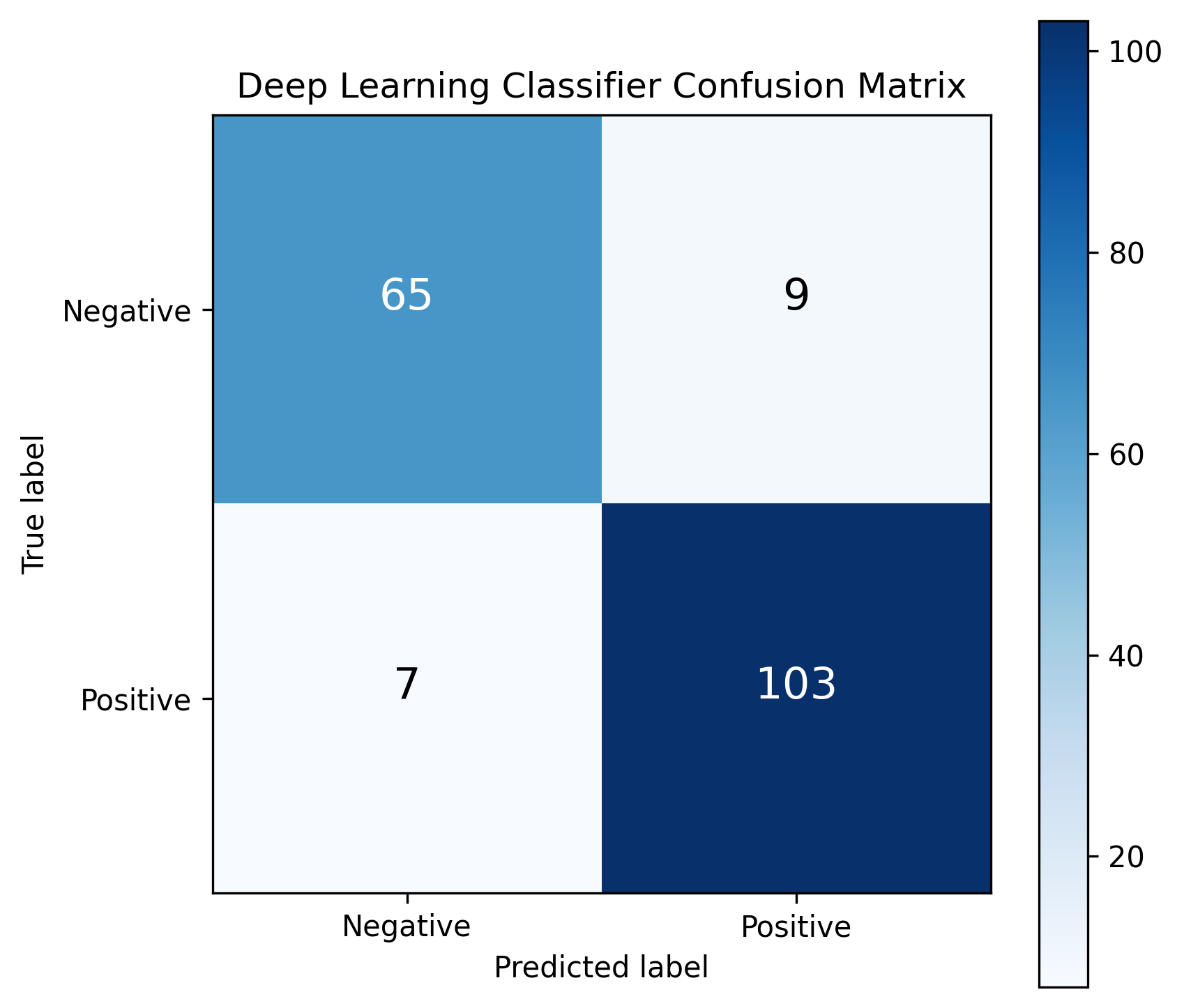
Deep Learning Model:
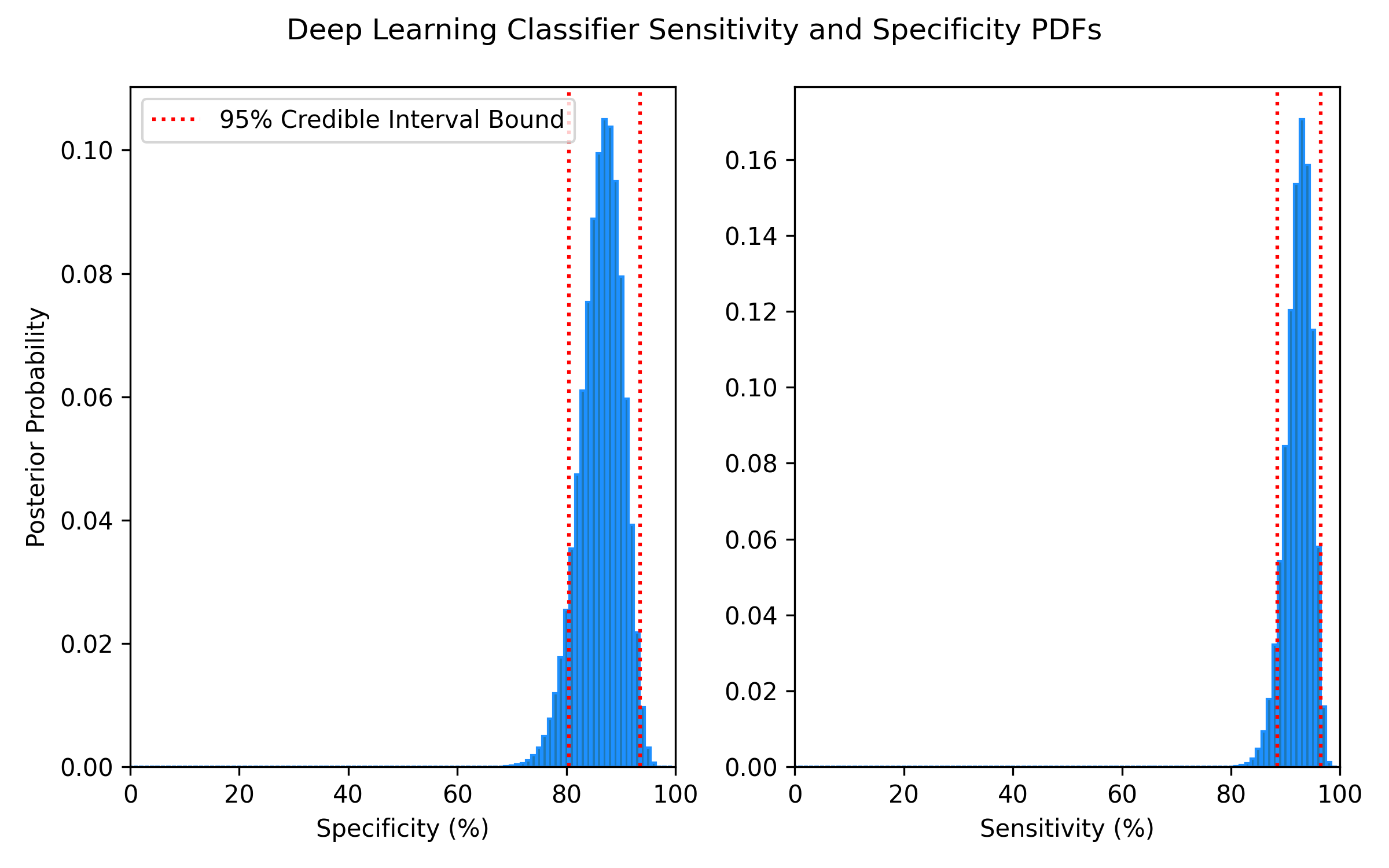
The top performing model by Accuracy, Recall, and F1-Score was a deep learning model trained on data where missing cholesterol values were imputed using the mean of the available values. Performance metrics can be found in the below figures and in Tables 1 and 2. To accompany the single-number metrics, PDFs were also constructed to quantify the uncertainty in this model’s sensitivity/recall and specificity. I wrote a comprehensive report detailing the generation of Sensitivity and Specificity PDFs and Credible Intervals which can be found in the repository, or by clicking this link
Table 1: Deep Learning Model Performance
Accuracy
Precision
Recall
F1-Score
Specificity
91.30%
91.96%
93.64%
92.79%
87.84%
Table 2: Deep Learning Model Sensitivity and Specificity CI
95% CI Minimum
95% CI Maximum
Sensitivity/Recall
88.5%
96.5%
Specificity
80.5%
93.5%
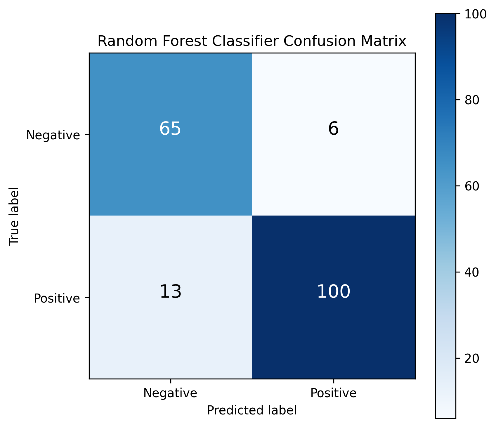
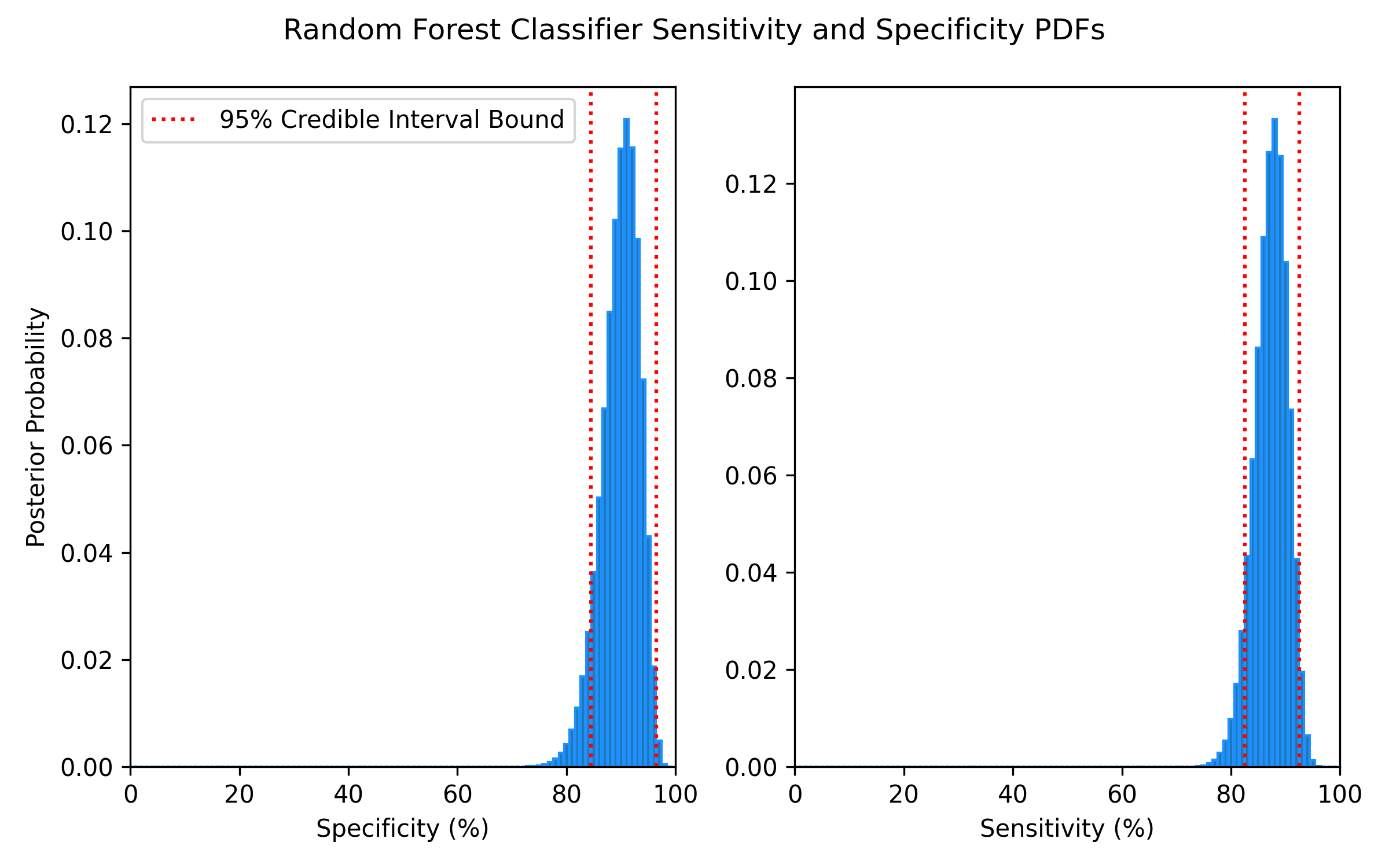
Random Forest Classifier:
The top performing model by Precision and Specificity was a Random Forest Classifier trained on data with missing cholesterol values imputed using Ridge Regression. Performance metrics can be found in the below figures and in Tables 2 and 3.
Table 3: Random Forest Classifier Performance
Accuracy
Precision
Recall
F1-Score
Specificity
89.67%
94.34%
88.50%
91.32%
91.55%
Table 4: Random Forest Classifier Sensitivity and Specificity CI
import*asieee754from"https://deno.land/x/ieee754/mod.ts";// or// import read from "https://deno.land/x/ieee754/read.ts";// import write from "https://deno.land/x/ieee754/write.ts";constbuf: Uint8Array=Uint8Array.of(0x42,0x29,0xae,0x14);constf64=ieee754.read(buf,0,false,52,8);console.log(f64);// 42.42constEPSILON=0.00001;constf32=ieee754.read(buf,0,false,23,4);console.log(Math.abs(f32-42.42)<EPSILON);// true
Use with number array:
constarr: number[]=[1,2,3];// a number arrayconstbuf=Uint8Array.from(arr);// convert to `Uint8Array`constnum=ieee754.read(buf,0,false,23,4);
APIs
read:
/** * Read IEEE754 floating point numbers from a array. * @param buffer the buffer * @param offset offset into the buffer * @param isLE is little endian? * @param mLen mantissa length * @param nBytes number of bytes */functionread(buffer: Uint8Array,offset: number,isLE: boolean,mLen: number,nBytes: number,): number;
write:
/** * Write IEEE754 floating point numbers to a array. * @param buffer the buffer * @param value value to set * @param offset offset into the buffer * @param isLE is little endian? * @param mLen mantissa length * @param nBytes number of bytes */functionwrite(buffer: Uint8Array,value: number,offset: number,isLE: boolean,mLen: number,nBytes: number,): void;
License
deno_ieee754 is released under the
MIT License. See the bundled LICENSE file for details.
Motivation: I have always thought that the only way to truely test if you understand a concept is to see if you can build it. As such all these these algorithms are implemented studying the relevant papers and coded to test my understanding.
What I cannot create, I do not understand” – Richard Feynman
These were mainly referenced from a really good lecture series by Colin Skow on youtube [link]. A large part was also found in the Deep Reinforcement Learning Udacity course.
Converged to an average of 17.56 after 1300 Episodes.
Code and results can be found under DQN/7. Vanilla DQN Atari.ipynb
DDPG Continuous
Converged to ~ -270 after a 100 episodes
Code and results can be found under Policy Gradient/4. DDPG.ipynb.ipynb
PPO discrete
Solved in 409 episodes
Code and results can be found under Policy Gradient/5. PPO.ipynb
PPO Atari – with Baseline Enhancements
Code and results can be found under PPO/
Todo
Curiousity Driven Exploration
HER (Hindsight Experience Replay)
Recurrent networks in PPO and DDPG
Credits
Whilst I tried to code everything directly from the papers, it wasn’t always easy to understand what I was doing wrong when the algorithm just wouldn’t train or I got runtime errors. As such I used the following repositories as references.
Script to apply some filters to BMP images. Written entirely in c ++.
Run it🚀
Just clone the project using git clone in the directory where you want to use the project. Once the project is cloned, the most important files you will have will be the “makefile” file and the code itself. In addition, certain sample images are also provided in an additional folder.
To run it you must have an input directory (the one we give as an example is valid) and an output directory (it can be the same as the input directory). Once this is cleared, simply type make in the terminal, in the root directory of the project. If there are no errors, continue entering the following command:
./img-par filter input_directory output_directory
If no errors appear, you should see the images from the input directory in the output directory, but with the specified filter applied.
Warning:This project is developed and thought to be compiled in a Linux environment. You must have the necessary environment to compile c++ files (using the g++ compiler). Other libraries may need installation, especially in case we want to work on windows
Posible filters📷
At the moment, only one of the following filters can be used:
Copy: The equivalent of not using any filter. The files will simply be copied from the input directory to the output directory. For example, when copying the following image of the tiger, we will obtain:
Gauss: In image processing, a Gaussian blur (also known as Gaussian smoothing) is the result of blurring an image by a Gaussian function. See wiki
Sobel: The Sobel operator, sometimes called the Sobel–Feldman operator or Sobel filter, is used in image processing and computer vision, particularly within edge detection algorithms where it creates an image emphasising edges. See wiki
To use one of these filters, just replace the word “filter” of the command from the previous section with the word of the corresponding filter.
Want to collaborate?🙋🏻
Feel free to try adding new filters, or improving and optimizing existing code. The sobel filter works a bit bad on certain edges of some images.
You can use it to submit your listening history to your ListenBrainz account with your own apps.
For end users, there is also the elbisaur CLI, which exposes many features of the library to the command line.
In addition to showcasing the usage of the API client, it also has advanced features to manage listens.
Features
Submits listens and playing now notifications
Browses your listening history and allows you to delete listens
Handles ListenBrainz authorization and API errors
Adheres to rate limits and optionally retries failed requests
Provides generic GET and POST methods for (yet) unsupported API endpoints
Includes additional parsers to extract listens from text formats
Ships with type definitions and inline documentation
As this library only makes use of web standards, it is also compatible with modern browsers (after transpilation to JavaScript).
Usage
In order to submit listens, you have to specify a user token which you can obtain from your ListenBrainz settings page.
The following example instantiates a ListenBrainz client with a token from an environment variable and submits a playing now notification for a track:
All listen parsers accept text input and generate Listen objects as their output.
These objects can then be used together with the ListenBrainz API and the LB client.
None of the parsers performs any filtering of listens, so you have to detect potential duplicates and skipped listens yourself.
The parsers do not include any logic to access files to make them platform independent.
You can pass them the content from a HTTP response body or from a file, for example.
The following parsers are available in the listenbrainz/parser/* submodules:
JSON: Accepts a JSON-serialized Listen object (as shown by the LB “Inspect listen” dialog) or an array of Listen objects as input.
JSONL: Multiple JSON-serialized Listen objects, separated by line breaks (format of listens files from a LB listening history export).
MusicBrainz: Accepts a release from the MusicBrainz JSON API and creates listens for the selected tracks.
.scrobbler.log: TSV table document which is generated by some portable music players for later submission to Last.fm.
Parser currently accepts files with AUDIOSCROBBLER/1.1 header which are generated by players with Rockbox firmware, possibly also by others.
Automatically converts timestamps from your local timezone to UTC (as Rockbox players are usually not timezone-aware).
Skipped listens are marked with track_metadata.additional_info.skipped = true.
Spotify: JSON files from an Extended Streaming History download.
Calculates the correct listen (start) timestamp from stream end time and duration.
Makes use of the “offline” timestamp to detect extreme outliers where Spotify has only logged a stream as ended when the app was next opened.
Skipped listens can be detected by their track_metadata.additional_info attributes skipped, reason_end and a too short duration_ms.
Translations in languages other than English are machine translated and are not yet accurate. No errors have been fixed yet as of March 21st 2021. Please report translation errors here. Make sure to backup your correction with sources and guide me, as I don’t know languages other than English well (I plan on getting a translator eventually) please cite wiktionary and other sources in your report. Failing to do so will result in a rejection of the correction being published.
Try it out! The sponsor button is right up next to the watch/unwatch button.
Version history
Version history currently unavailable
No other versions listed
Software status
All of my works are free some restrictions. DRM (Digital Restrictions Management) is not present in any of my works.
This sticker is supported by the Free Software Foundation. I never intend to include DRM in my works.
I am ussing the abbreviation “Digital Restrictions Management” instead of the more known “Digital Rights Management” as the common way of addressing it is false, there are no rights with DRM. The spelling “Digital Restrictions Management” is more accurate, and is supported by Richard M. Stallman (RMS) and the Free Software Foundation (FSF)
This section is used to raise awareness for the problems with DRM, and also to protest it. DRM is defective by design and is a major threat to all computer users and software freedom.


 https://github.com/Flo-Schilli/ha-grohe_smarthome