Translations in languages other than English are machine translated and are not yet accurate. No errors have been fixed yet as of March 21st 2021. Please report translation errors here. Make sure to backup your correction with sources and guide me, as I don’t know languages other than English well (I plan on getting a translator eventually) please cite wiktionary and other sources in your report. Failing to do so will result in a rejection of the correction being published.
Try it out! The sponsor button is right up next to the watch/unwatch button.
Version history
Version history currently unavailable
No other versions listed
Software status
All of my works are free some restrictions. DRM (Digital Restrictions Management) is not present in any of my works.
This sticker is supported by the Free Software Foundation. I never intend to include DRM in my works.
I am ussing the abbreviation “Digital Restrictions Management” instead of the more known “Digital Rights Management” as the common way of addressing it is false, there are no rights with DRM. The spelling “Digital Restrictions Management” is more accurate, and is supported by Richard M. Stallman (RMS) and the Free Software Foundation (FSF)
This section is used to raise awareness for the problems with DRM, and also to protest it. DRM is defective by design and is a major threat to all computer users and software freedom.
Welcome to the Maintenance App,This platform that enables faculty and staff at University of Jaffna to submit maintenance requests for campus buildings and facilities.With this app, users can quickly and easily create a complaint, which will be assigned to a work engineer for review and resolution. The app allows for efficient tracking of maintenance requests, ensures timely follow-up, and streamlines communication between the university and its community.
Technologies Used
This app is built using the MERN stack, which includes:
MongoDB: a NoSQL database for storing and managing data
Express.js: a Node.js framework for building web applications
React Native: a front-end JavaScript library for building user interfaces
Node.js: a JavaScript runtime environment for executing server-side code
Features
User Authentication: Secure login system for users, work engineers, and supervisors
Complaint Submission: Users can create a complaint with details of the issue, and add images if necessary
Complaint Assignment: Work engineers can view all complaints and assign them to supervisors for review
Complaint Tracking: Supervisors can track the progress of assigned complaints, update their status, and add comments
Notifications: Automated email notifications for complaint submission, assignment, and resolution
Admin Panel: For managing users, work engineers, supervisors, and complaint categories
Installation and Setup
To get started with the Maintenance App, follow these steps:
Integrative Methods of Analysis for Genetic Epidemiology
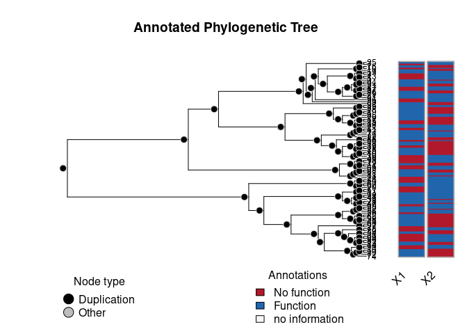
geese: GEne-functional Evolution using SufficiEncy
This R package taps into statistical theory primarily developed in
social networks. Using Exponential-Family Random Graph Models (ERGMs),
geese provides a statistical framework for building Gene Functional
Evolution Models using Sufficiency. For example, users can directly
hypothesize whether Neofunctionalization or Subfunctionalization events
were taking place in a phylogeny, without having to estimate the full
transition Markov Matrix that is usually used.
GEESE is computationally efficient, with C++ under the hood, allowing
the analyses of either single trees (a GEESE) or multiple trees
simultaneously (pooled model) in a Flock.
This is a work in progress and based on the theoretical work developed
during George G. Vega Yon’s doctoral thesis.
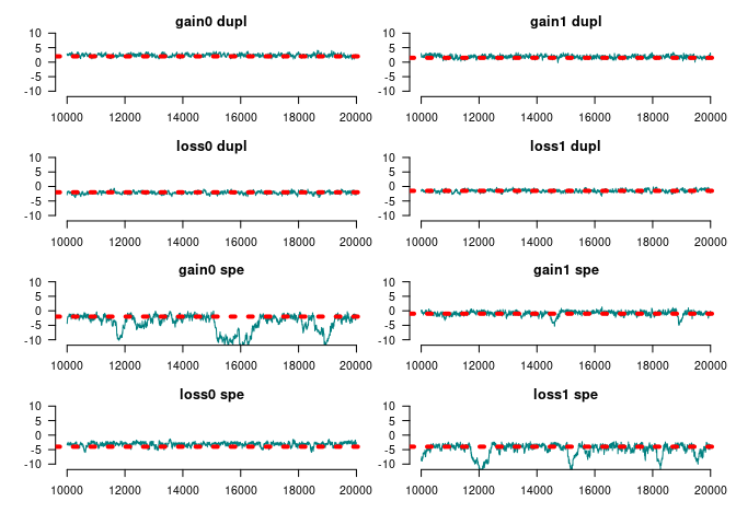
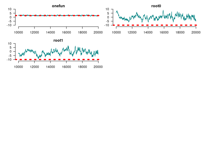
#>
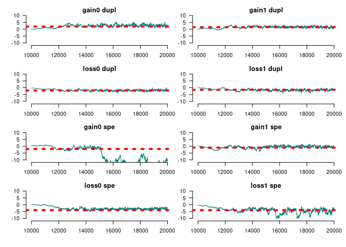
#> Iterations = 15000:20000
#> Thinning interval = 1
#> Number of chains = 1
#> Sample size per chain = 5001
#>
#> 1. Empirical mean and standard deviation for each variable,
#> plus standard error of the mean:
#>
#> Mean SD Naive SE Time-series SE
#> Gains 0 at duplication 2.9015 0.8051 0.011385 0.09034
#> Gains 1 at duplication 1.6914 0.5653 0.007994 0.04934
#> Loss 0 at duplication -2.0287 0.5349 0.007563 0.05280
#> Loss 1 at duplication -1.8866 0.6442 0.009110 0.08533
#> Gains 0 at speciation -12.1932 3.5435 0.050107 1.15176
#> Gains 1 at speciation -0.1454 0.6609 0.009345 0.06815
#> Loss 0 at speciation -2.9909 0.5184 0.007331 0.04458
#> Loss 1 at speciation -5.1655 1.9408 0.027444 0.39515
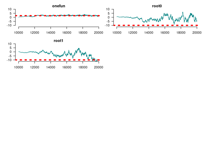
#> Genes with [0, 1] funs 2.2578 0.4569 0.006461 0.06265
#> Root 1 -1.0470 3.0807 0.043564 0.94842
#> Root 2 -4.2756 4.2474 0.060061 1.59284
#>
#> 2. Quantiles for each variable:
#>
#> 2.5% 25% 50% 75% 97.5%
#> Gains 0 at duplication 1.4054 2.3030 2.8777 3.4337 4.5624
#> Gains 1 at duplication 0.5451 1.3327 1.7001 2.0905 2.7559
#> Loss 0 at duplication -3.0657 -2.3764 -2.0460 -1.6762 -0.9765
#> Loss 1 at duplication -3.1944 -2.3389 -1.8797 -1.4119 -0.6868
#> Gains 0 at speciation -18.2113 -14.9130 -12.1597 -10.1648 -3.6030
#> Gains 1 at speciation -1.5472 -0.5998 -0.1365 0.3416 1.0736
#> Loss 0 at speciation -4.0181 -3.3470 -2.9738 -2.6539 -2.0354
#> Loss 1 at speciation -9.4815 -6.5157 -4.8115 -3.6121 -2.3045
#> Genes with [0, 1] funs 1.4263 1.9483 2.2481 2.5599 3.2238
#> Root 1 -5.9435 -3.5719 -1.4757 1.4858 4.7924
#> Root 2 -14.2253 -5.9892 -3.8179 -1.5920 3.3555
par_estimates<- colMeans(
window(ans_mcmc, start= end(ans_mcmc)*3/4)
)
ans_pred<- predict_geese(
amodel, par_estimates,
leave_one_out=TRUE,
only_annotated=TRUE
) |> do.call(what="rbind")
# Preparing annotationsann_obs<- do.call(rbind, fake1)
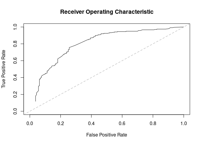
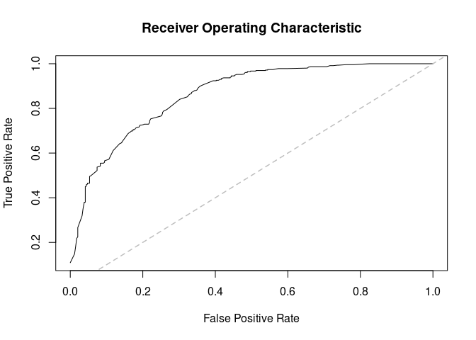
# AUC
(ans<- prediction_score(ans_pred, ann_obs))
#> Prediction score (H0: Observed = Random)#> #> N obs. : 199#> alpha(0, 1) : 0.40, 0.60#> Observed : 0.68 ***#> Random : 0.52 #> P(<t) : 0.0000#> --------------------------------------------------------------------------------#> Values scaled to range between 0 and 1, 1 being best.#> #> Significance levels: *** p < .01, ** p < .05, * p < .10#> AUC 0.80.#> MAE 0.32.
plot(ans$auc, xlim= c(0,1), ylim= c(0,1))
Using a flock
GEESE models can be grouped (pooled) into a flock.
flock<- new_flock()
# Adding first set of annotations
add_geese(
flock,
annotations=fake1,
geneid= c(tree[, 2], n),
parent= c(tree[, 1],-1),
duplication=duplication
)
# Now the second set
add_geese(
flock,
annotations=fake2,
geneid= c(tree[, 2], n),
parent= c(tree[, 1],-1),
duplication=duplication
)
# Persistence to preserve parent state
term_gains(flock, 0:1, duplication=1)
term_loss(flock, 0:1, duplication=1)
term_gains(flock, 0:1, duplication=0)
term_loss(flock, 0:1, duplication=0)
term_maxfuns(flock, 0, 1, duplication=2)
# We need to initialize to do all the accountintg
init_model(flock)
#> Initializing nodes in Flock (this could take a while)...#> ||||||||||||||||||||||||||||||||||||||||||||||||||||||||||||||||||||||||| done.
print(flock)
#> FLOCK (GROUP OF GEESE)#> INFO ABOUT THE PHYLOGENIES#> # of phylogenies : 2#> # of functions : 2#> # of ann. [zeros; ones] : [165; 235]#> # of events [dupl; spec] : [86; 112]#> Largest polytomy : 2#> #> INFO ABOUT THE SUPPORT#> Num. of Arrays : 792#> Support size : 8#> Support size range : [1, 1]#> Transform. Fun. : no#> Model terms (9) :#> - Gains 0 at duplication#> - Gains 1 at duplication#> - Loss 0 at duplication#> - Loss 1 at duplication#> - Gains 0 at speciation#> - Gains 1 at speciation#> - Loss 0 at speciation#> - Loss 1 at speciation#> - Genes with [0, 1] funs
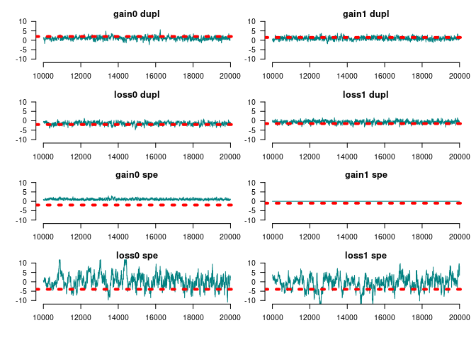
summary(window(ans_mcmc2, start=10000))
#> #> Iterations = 10000:20000#> Thinning interval = 1 #> Number of chains = 1 #> Sample size per chain = 10001 #> #> 1. Empirical mean and standard deviation for each variable,#> plus standard error of the mean:#> #> Mean SD Naive SE Time-series SE#> Gains 0 at duplication 2.39204 0.4707 0.004707 0.03019#> Gains 1 at duplication 1.85804 0.4925 0.004925 0.02789#> Loss 0 at duplication -2.15114 0.4451 0.004451 0.03310#> Loss 1 at duplication -1.50477 0.4427 0.004427 0.03176#> Gains 0 at speciation -4.10744 2.9954 0.029952 0.76564#> Gains 1 at speciation -0.84969 0.8242 0.008241 0.09520#> Loss 0 at speciation -3.16554 0.6535 0.006535 0.05307#> Loss 1 at speciation -4.88115 2.0161 0.020160 0.32971#> Genes with [0, 1] funs 2.09933 0.3703 0.003702 0.02921#> Root 1 0.02501 2.6487 0.026486 0.45210#> Root 2 -1.07238 2.9197 0.029195 0.56841#> #> 2. Quantiles for each variable:#> #> 2.5% 25% 50% 75% 97.5%#> Gains 0 at duplication 1.5050 2.068 2.37614 2.7239 3.3368#> Gains 1 at duplication 0.9237 1.511 1.84256 2.2029 2.8299#> Loss 0 at duplication -3.0413 -2.451 -2.14564 -1.8533 -1.2836#> Loss 1 at duplication -2.3961 -1.809 -1.51894 -1.1984 -0.6178#> Gains 0 at speciation -11.2547 -5.414 -2.91312 -1.9486 -0.9131#> Gains 1 at speciation -3.2320 -1.183 -0.72227 -0.3283 0.3280#> Loss 0 at speciation -4.7209 -3.510 -3.08984 -2.7347 -2.0557#> Loss 1 at speciation -10.5227 -5.326 -4.19469 -3.5823 -2.7532#> Genes with [0, 1] funs 1.3738 1.842 2.07762 2.3515 2.8303#> Root 1 -4.7967 -1.873 -0.04377 1.5864 6.0565#> Root 2 -6.5355 -3.147 -1.08668 1.1586 4.6030
Are we doing better in AUCs?
par_estimates<- colMeans(
window(ans_mcmc2, start= end(ans_mcmc2)*3/4)
)
ans_pred<- predict_flock(
flock, par_estimates,
leave_one_out=TRUE,
only_annotated=TRUE
) |>
lapply(do.call, what="rbind") |>
do.call(what=rbind)
# Preparing annotationsann_obs<- rbind(
do.call(rbind, fake1),
do.call(rbind, fake2)
)
# AUC
(ans<- prediction_score(ans_pred, ann_obs))
#> Prediction score (H0: Observed = Random)#> #> N obs. : 398#> alpha(0, 1) : 0.42, 0.58#> Observed : 0.72 ***#> Random : 0.51 #> P(<t) : 0.0000#> --------------------------------------------------------------------------------#> Values scaled to range between 0 and 1, 1 being best.#> #> Significance levels: *** p < .01, ** p < .05, * p < .10#> AUC 0.86.#> MAE 0.28.
plot(ans$auc)
Limiting the support
In this example, we use the function rule_limit_changes() to apply a
constraint to the support of the model. This takes the first two terms
(0 and 1 since the index is in C++) and restricts the support to states
where there are between $[0, 2]$ changes, at most.
This should be useful when dealing with multiple functions or
pylotomies.
# Creating the objectamodel_limited<- new_geese(
annotations=fake1,
geneid= c(tree[, 2], n),
parent= c(tree[, 1],-1),
duplication=duplication
)
# Adding the model terms
term_gains(amodel_limited, 0:1)
term_loss(amodel_limited, 0:1)
term_maxfuns(amodel_limited, 1, 1)
term_overall_changes(amodel_limited, TRUE)
# At most one gain
rule_limit_changes(amodel_limited, 5, 0, 2)
# We need to initialize to do all the accounting
init_model(amodel_limited)
#> Initializing nodes in Geese (this could take a while)...#> ||||||||||||||||||||||||||||||||||||||||||||||||||||||||||||||||||||||||| done.# Is limiting the support any useful?
support_size(amodel_limited)
#> [1] 31
Since we added the constraint based on the term
term_overall_changes(), we now need to fix the parameter at 0 (i.e.,
no effect) during the MCMC model:
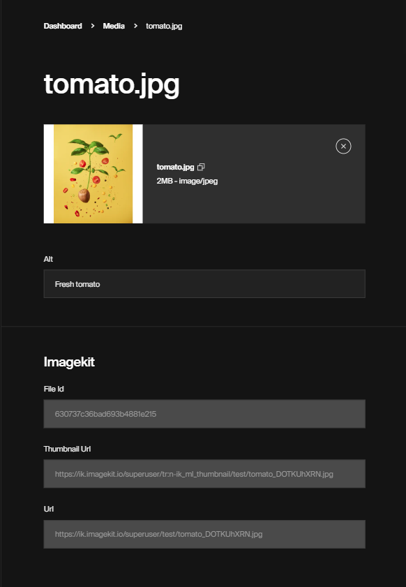
Install this plugin within your Payload as follows:
import{buildConfig}from"payload/config";importimagekitPluginfrom"payloadcms-plugin-imagekit";exportdefaultbuildConfig({// ...plugins: [imagekitPlugin({config: {publicKey: "your_public_api_key",privateKey: "your_private_api_key",endpoint: "https://ik.imagekit.io/your_imagekit_id/",},collections: {media: {uploadOption: {folder: "some folder",extensions: [{name: "aws-auto-tagging",minConfidence: 80,// only tags with a confidence value higher than 80% will be attachedmaxTags: 10,// a maximum of 10 tags from aws will be attached},{name: "google-auto-tagging",minConfidence: 70,// only tags with a confidence value higher than 70% will be attachedmaxTags: 10,// a maximum of 10 tags from google will be attached},],},savedProperties: ["url","AITags"],},},}),],});
Plugin options
This plugin have 1 parameter that contain an object.
Option
Description
config (required)
ImageKit Config ImageKitOptions
collections (optional)
Collections options
config
Type object
publicKey: type string
privateKey: type string
endpoint: type string;
collections
Type object
[key] (required)
type: string
description: Object keys should be PayloadCMS collection name that store the media/image.
value type: object
value options:
uploadOption (optional)
type: object
type detail: TUploadOption. Except file.
description: An options to saved in ImageKit.
savedProperties (optional)
type: []string
type detail: TImageKitProperties. Except thumbnailUrl and fileId.
description: An object that saved to PayloadCMS/Database that you may need it for your Frontend.
disableLocalStorage (optional)
type: boolean
default: true
description: Completely disable uploading files to disk locally. More
Payload Cloud
If your project is hosted using Payload Cloud – their default file storage solution will conflict with this plugin. You will need to disable file storage via the Payload Cloud plugin like so:
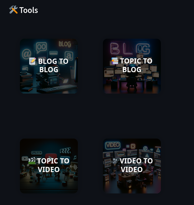
noobies.ai is an open-source project designed to empower users in AI-driven content generation. It provides an extensive set of tools for creating diverse content, including blogs, images, videos, and audio. The project aims to simplify AI-based content creation while ensuring accessibility and user-friendliness.
Screenshots
Features
Blog Generation
The project includes a powerful blog generation module, allowing users to effortlessly create engaging written content.
fromnoobies_ai.coreimportblog_generator# Example usagegenerated_blog=blog_generator.generate_blog(topic="AI in 2024")
Video Generation
Generate dynamic video content with ease using the video generation module.
fromnoobies_ai.coreimportvideo_generator# Example usagegenerated_video=video_generator.generate_video(topic="Future Technologies")
AI Utilities
ImageAI
Harness the power of ImageAI to process and analyze images.
fromnoobies_ai.core.utils.AIimportimageAI# Example usageimage_labels=imageAI.process_image("path/to/image.jpg")
TextAI
Generate AI-driven text content effortlessly.
fromnoobies_ai.core.utils.AIimporttextAI# Example usagegenerated_text=textAI.generate_text(prompt="Describe a futuristic city.")
AudioAI
Explore the capabilities of AudioAI for audio-related tasks.
fromnoobies_ai.core.utils.AIimportaudioAI# Example usagetranscription=audioAI.transcribe_audio("path/to/audio.mp3")
Content Conversion
Convert content seamlessly between different formats.
fromnoobies_ai.core.utils.converterimportblog_converter, image_converter, video_converter# Example usageconverted_blog=blog_converter.convert_to_blog(generated_text)
converted_image=image_converter.convert_to_image(generated_blog)
converted_video=video_converter.convert_to_video(generated_text)
app.py: Main application script using Streamlit for the user interface.
Streamlit Application
The primary interface for interacting with noobies.ai is a Streamlit web application. Follow these steps to run the application locally:
Install dependencies:
pip install -r requirements.txt
Run the Streamlit app:
streamlit run app.py
This will launch the application in your default web browser.
Explore the Features:
Navigate through the different sections of the application to explore and use the various content generation features. Interact with the intuitive user interface to leverage the power of AI in content creation.
Usage Examples
Blog Generation
fromnoobies_ai.coreimportblog_generator# Example usagegenerated_blog=blog_generator.generate_blog(topic="AI in 2024")
Dependencies
Ensure you have the required dependencies installed by running:
pip install -r requirements.txt
Contributing
We welcome contributions! Feel free to open issues, submit pull requests, or provide feedback.
Exploring Customer Segmentation and Customer Lifetime Value for Sales Forecasting
Background
Welcome to the data exploration journey of understanding customer behavior and enhancing sales forecasting for a UK-based company specializing in unique all-occasion gifts. Our goal is to unlock valuable insights from customer data and historical sales, laying the foundation for effective customer segmentation and improved sales predictions.
Objectives
Understand the Data:
Dive deep into the provided Online Retail II dataset to comprehend its intricacies and features.
Exploratory Data Analysis (EDA):
Perform comprehensive exploratory data analysis to uncover hidden patterns, trends, and anomalies within the dataset.
Data Preparation:
Preprocess and prepare the data for subsequent analyses, ensuring its suitability for modeling.
Customer Segmentation:
Utilize advanced segmentation techniques to categorize customers based on their behavior, preferences, and historical interactions.
Forecasting Models:
Develop and implement tailored forecast models for each customer segment, aiming for accurate sales predictions.
Results Presentation:
Present the findings, insights, and actionable recommendations in a clear and concise manner.
Data Description
The heart of our exploration lies in the Online Retail II dataset, offering a real-world snapshot of online retail transactions. The primary data elements include:
online_retail_II.xlsx
This comprehensive table captures records for all created orders, boasting 1,067,371 rows and 8 columns. With a size of 44.55MB, it serves as a rich source of information for our analysis.
Data Element
Type
Description
Invoice
object
Invoice number, uniquely assigned to each transaction. If starting with ‘c’, it signifies a cancellation.
StockCode
object
Unique product (item) code assigned to each distinct product.
Description
object
Descriptive name of the product (item).
Quantity
int64
Quantities of each product (item) per transaction.
InvoiceDate
datetime
Date and time of the invoice generation.
Price
float64
Unit price of the product in pounds (£).
Customer ID
int64
Unique customer identifier with a 5-digit integral number.
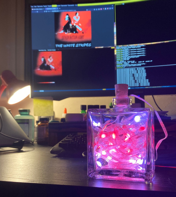
I got a Pimoroni Wireless Plasma Kit and wanted to do something fun with it! I had the idea to create a custom palette of colors based on what I was listening to!
Album art is often iconic and I thought it’d be cool to get a subtle hint of the colors of my favorite album covers as their songs play!
I realized that last.fm shares album art over its API and as a long time member, that seemed like a great place to start.
By combining code for API access, dominant color extraction, NeoPixel updates and socket networking I was able to throw this together in an evening.
Materials
A last.fm account to pull from w/ API key
A ‘server’ (such as a Raspberry Pi Pico) to talk to the LEDs
Plays music / can obtain the currently playing song (eg mpc/mpd)
Generate color palettes via API calls
[Optionally] detects BPM (via eg bpm from bpm-tools)
Workflow
I really wish the pico could do all of the image processing but jpeg decoding let alone kmeans is probably a tall order…so I arrived at this slightly hacky client/server architecture.
The client code (running on a ‘real’ computer) does most of the heavy lifting by:
Checking last.fm for the most recently scrobbled track
Downloading it’s cover art
Extract the NUM_COLORS most common colors
Padding that out to NUM_LEDS and sending the udpdate to the server.
Here’s what that looks like, in the client’s terminal; note the track name, album art visualization and palette preview:
(There are now 4 palette extraction algorithms and all of them are previewed though only one is sent to the server!)
The server code, running on the pico, is resonsible for:
Accepting “palette” updates (which are a list of NUM_LED RGB values)
Managing the LED colors
Running the project
Have a look at the constants at the top of the client / server and see if you wanna make any adjustments
Install the libraries in requirements.txt on your client
Use thonny or something like it to run the server code on the pi
It’ll glow green when it’s ready for a client connection
Run the client code (once you add the API key and username) on a ‘real’ computer to send palettes to the server
Good Stuff
Proud of janky palette transition logic; exciting when songs switch!
Gentle animation is nice
Because the pico has wifi, it can be anywhere in your home! On a high shelf, even. Wireless is cool 🙂
The updates are pretty slick
Once a palette has been recieved it’ll keep on displaying it until a new one is recieved.
Pretty pleased by the threading code on the pico for handling animation and network updates 🙂
BPM support
If you set a BPM_CMD you should be able to have the lights pulse at the BPM of the audio!
I use a shell script like this:
#!/bin/bash
BPMPATH=`which bpm`
FFMPEGPATH=`which ffmpeg`
BCPATH=`which bc`
BASE=/mnt/media/music/music
PATH=`mpc status --format "%file%"| head -n1`
FULLPATH=$BASE/$PATH# convert to raw audio using ffmpeg + measure bpm!# Thanks to Mark Hills for `bpm` and https://gist.github.com/brimston3/34dbb439442a723313b019b92931887b !
bpm=$($FFMPEGPATH -hide_banner -loglevel error -vn -i "$FULLPATH" -ar 44100 -ac 1 -f f32le pipe:1 |$BPMPATH)#echo "BPM=$bpm"# Calculate Delay
delay=$($BCPATH -l <<<60.0/$bpm)#echo "Delay=$delay"echo$delay
Future Work
Here are a few ideas I have for future improvements…
Client:
Automatically choose the best number of clusters?
TUI interace:
q for quit
1,2,3,4 etc for different color extraction methods?
cache recent songs:
can’t really cache checks with last.fm; move to a model where we search last.fm for the song on change?
API retries?
more interesting fake patterns if missing a song!
extract hues rather than brightnesses?
Server:
It’s possible having all the LEDs stuff into a bottle isn’t given the best sense of the palette — might look cool mounted on a wall or somewhere else!
(train) lantern?
Mount them along a wall or around a window frame?
More interesting animation patterns?
create multiple “endpoints” for various controls
changing animation speed?
explicitly set LEDs
test pattern?
Bugs to fix:
Traceback (most recent call last):
  File "/home/jesse/projects/album_art_bottle_LEDs/plasma_client.py", line 3
40, in <module>
    main()
  File "/home/jesse/projects/album_art_bottle_LEDs/plasma_client.py", line 3
21, in main
    colors = generate_palette(session, methods)
             ^^^^^^^^^^^^^^^^^^^^^^^^^^^^^^^^^^
  File "/home/jesse/projects/album_art_bottle_LEDs/plasma_client.py", line 2
45, in generate_palette
    payload = get_info_from_last_scrobble()
              ^^^^^^^^^^^^^^^^^^^^^^^^^^^^^
  File "/home/jesse/projects/album_art_bottle_LEDs/plasma_client.py", line 1
55, in get_info_from_last_scrobble
    last_track = response.json()['recenttracks']['track'][0]
                 ~~~~~~~